
Temper, Temper: A steelmaker's solution to take the swing out of AI training loads
AI training loads are electric arc furnaces; this one is a first-principle buffering formula for AI training loads, borrowed from steelmaking

We’ve slowly turned our back on our steelmaking heritage in the UK, but there’s still a small thread left. That’s Tata’s £1.25bn electric arc furnace at Port Talbot. The data centre crowd could empathise with their woes also, because the plant at Port Talbot is is currently running about twelve months late, waiting on power.
This is because National Grid can’t energise the Margam connection in time; a new 275kV gas-insulated substation, a second 275kV substation inside the steelworks, supergrid transformers and two kilometres of underground cable, all for one furnace.
That’s going to be a lot of power. Meanwhile, in tandem, there’s 50GW or so of data centre demand now sat in the UK connection queue, stuck in the same bottleneck.
Both are enormous loads, and are actually more similar than different. Both need electricity, and lots of it. But more importantly, both demands swing violently – the energy demand to get the furnace up to temperature requires monolithic amounts of energy. But once it’s up to temperature, that demand tails off. Same with AI loads – training loads are those which get the headlines about colossal energy consumption. Inference loads are still not insignificant, but are considerably less.
And yet still, both are asking for their buckets of power to be served by an ancient network built for a few kettles and some street lighting.
The difference is that steelmaking has a century of experience behind it, and the other is currently improvising.
So this is my argument for today; AI training loads are electric arc furnaces. Not loosely, nor metaphorically; in the specific electrical sense that matters to a grid planner. Thousands of GPUs run the same training iteration in lockstep, so compute-heavy and communication-heavy phases alternate across the whole cluster at once, and the site’s draw slams up and down by tens of megawatts in under a second.
That’s basically the same definition of a furnace. But steelmakers have already grappled with this issue. And they’ve written the maths down, put it in an international standard, and made the fix a condition of connection.
This isn’t the first time I’ve used a parallel universe to give a bit of data centre insight, so I may as well stay on-brand. Probably going to be full of flaws and plenty of holes in the argument – but nothing better seems to be getting suggested, so let’s run the steel protocol forwards and see what number falls out. I’ll carry one example the whole way through the rest of it: a generic 100MW AI-training hall.
Bore-in, bore-out
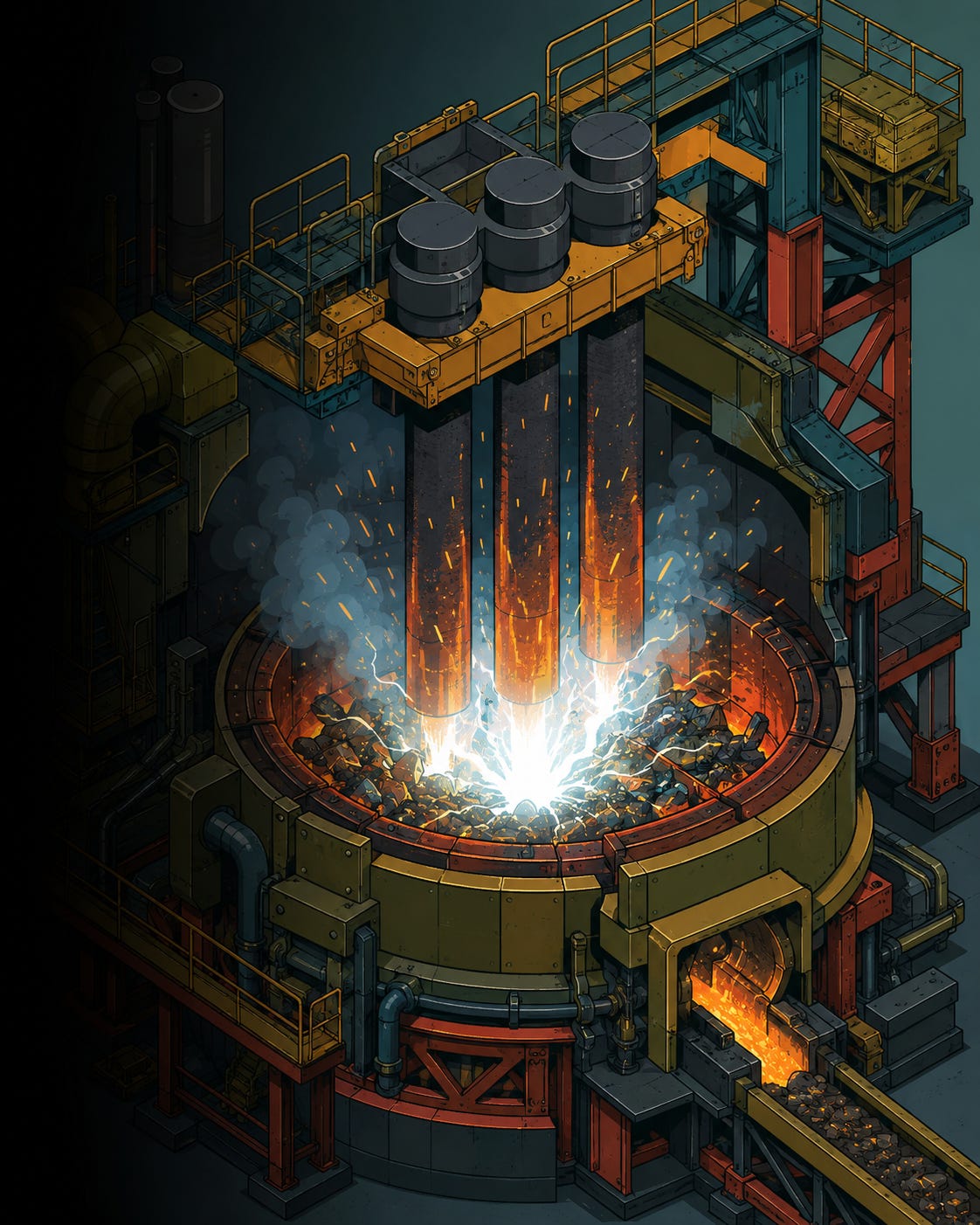
A modern arc furnace is 100 to 150MVA of transformer feeding three graphite electrodes into a bucket of cold scrap. During the bore-in phase, as the electrodes cut down through the pile, the arc strikes, collapses, re-strikes and wanders. The load goes from something close to a short circuit to something close to an open circuit, and back, continuously. The characteristic frequency content of that thrashing sits at roughly 4 to 14Hz.
That band is not a coincidence in the history of this problem. The human eye’s sensitivity to modulated light peaks at around 8.8Hz, and at that frequency you can perceive brightness modulation of well under half a percent. So when steelworks scaled up in the early twentieth century, the complaint that landed wasn’t from a systems engineer, btu from people whose lights were pulsing in their homes. Funnily enough, the entire discipline is still called “flicker” because of it.
The steel industry built a that tied to the strength of the connection, and published it. IEC 61000-3-7 gives the working relationship for a furnace’s flicker emission at the point of common coupling:
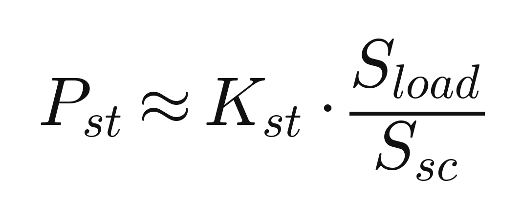
Pst is short-term flicker severity, where 1.0 is roughly the threshold of irritation for a typical observer. S_load is the furnace rating. S_sc is the short-circuit power available at the point of common coupling, which is the honest measure of how stiff your connection is. Kst is an empirical fudge factor that generally summarises how badly a given furnace actually thrashes; the standard puts it between 48 and 85 depending on the nature, weight and density of the scrap you’re melting, with 58 to 70 recommended for estimating (and 85 used for stainless).
Rearrange it against a planning level of Pst = 0.9 and you get the connection rule that has governed steel siting for decades:
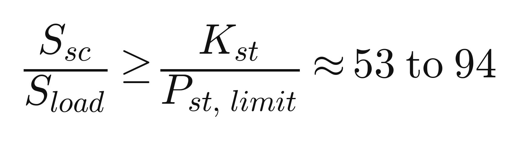
Sorry if you’re lost already (I had to read it about 10 times aswell, and I’m still barely grasping it…) so just fixate on this bit:
Your connection point needs somewhere between fifty and a hundred times more short-circuit power than your furnace has rating.
As I understand it, this is the whole reason Port Talbot it getting its own 275kV substation instead of just a feeder off the local network.
Stiff competition
I’m sure every steelworks electrical engineer in the industry knows their short-circuit ratio. Strangely though, I have never once seen a data centre planning document mention it. We talk about MW, we talk about PUE, we’ve started talking about WUE (I’ve got my own thoughts on that here), and we discuss critical load as though a megawatt were a megawatt (I’ve explained more nuance of this definition in turning crypto mines into data centres here).
This is basically suggesting that most planners treat the the strength of the network behind the meter as someone else’s problem that won’t affect them.
As I’m completely playing with this concept, if we invert the steel rules - it becomes a headroom allowance instead of a limit. If a fluctuating load can sit at up to about 1.5% of the short-circuit power at its connection point before it becomes a nuisance (which is what Pst = 0.9 with Kst = 60 works out to), then a site’s free allowance is:
ΔP_allow = ε × S_sc, with ε ≈ 1.5%
[Note, that transposition is mine rather than the standard’s – my maths could be crap, so double check it…]
My understanding is that Kst is usuakky calibrated on furnaces whose swing is roughly their own rating, so using it as though S_load were the swing amplitude is fair for a furnace; but probably needs checking for anything else. But that’s more of a design heuristic, not a compliance calculation.
It still gives you something the data centre industry doesn’t currently have: a defensible answer to “how much am I allowed to wobble”, set by the physics of the connection rather than by whatever the utility feels like writing into the agreement that week.
We come back to the same argument, and the same ‘flicker’ phenomenon – doesn’t matter what the agreement says; if people’s lights start flickering, then you’ve got to do something about it. And by that point, all of your investment has been made into something which now may need to be restricted or curtailed.
Reactive measures
The voltage disturbance a fluctuating load creates is approximately (ΔP·R + ΔQ·X)/V². On a high-voltage network, reactance dominates resistance by a wide margin, so the term that does the damage is ΔQ; the reactive swing. And an arc furnace’s disturbance is overwhelmingly reactive, because what’s changing is the impedance of the arc itself.
Which is why the steel industry’s solution is so cheap. A static VAr compensator, or a modern STATCOM, injects and absorbs reactive power in opposition to the furnace. The first commercial one went in back in 1964, using a saturated reactor to stop lamps flickering; thyristor control arrived in the 1970s and the technology has been routine ever since. Crucially, a STATCOM isn’t storing energy in any meaningful quantity. As I understand it, it’s basically shuffling phase. The DC capacitor inside it is small because reactive power doesn’t have to come from anywhere; you can conjure VArs out of switching.
So this is the data centre parallel challenge, and where my metaphor’s holes start to appear -because you cannot ‘conjure’ watts.
A data centre’s power supplies are power-factor corrected to around 0.99. When a training cluster drops out of its compute phase, what disappears is real power. There is no compensator that can fix that, because those joules have to come from somewhere physical.
So we’ve got to be careful about what we steal from steel (I’ve been waiting all article to use that one…):
Steel gives us the metric, the standard, the siting rule and the commercial model; but sadly, withholds the entire thing that made it all affordable.
There’s a second, and probably more impending problem. Arc furnaces thrash at 4 to 14Hz. AI training, according to the NVIDIA, Microsoft and OpenAI power stabilisation paper, has its FFT energy concentrated between 0.2 and 3Hz. That’s below the eye’s sensitivity peak, so the lights effectively barely move (hence you won’t see the ‘flicker’). It is also, precisely, the electromechanical band: below 1Hz you’re in the natural modes of long transmission lines, and 1 to 2.5Hz is where closely coupled generating plant oscillates against itself. The paper’s authors are blunt about the risk of exciting turbine-generator shaft torsional modes and sub-synchronous resonance, and cite a 2019 Florida event in which a single unstable combined-cycle unit set the system ringing with a driving magnitude of around 200MW.
A gigawatt of synchronised training load is five times that amount, and all happening at a frequency the eye can’t see and the shaft can feel.
So in simple terms: if there was a problem with steelmaking, you saw it or heard it. With AI equipment, you can’t. So by the time a problem is realized, it’s probably too late and your equipment and infrastructure has destroyed itself.
Joules in the crown
But back to the useful stuff we could use. To ensure our AI stuff doesn’t destroy itself, we can do the thing that steelmakers also do – factor in a buffer.
The buffering requirement has to be denominated in energy, and the derivation is simpler than it looks.
Model the iteration ripple as a sinusoid of peak-to-peak amplitude, ΔP at frequency, f. Integrate over the half cycle in which the load sits above its mean and you get ΔP/2πf, which is the energy the buffer has to hold. Subtract the amplitude the grid will accept for free, divide by round-trip efficiency, and you have it: (I’m fully aware that derivation wasn’t simple, I had to dig out my A-Level maths textbook to remind myself how to integrate).
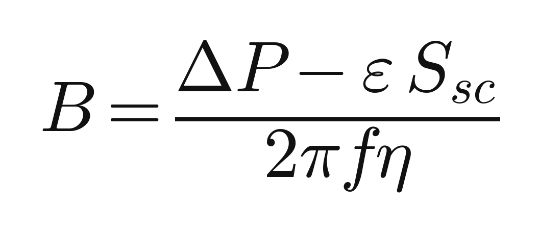
Normalise by site load and the result is more elegant than I expected. With α as the swing depth as a fraction of load, and SCR as the short-circuit ratio:
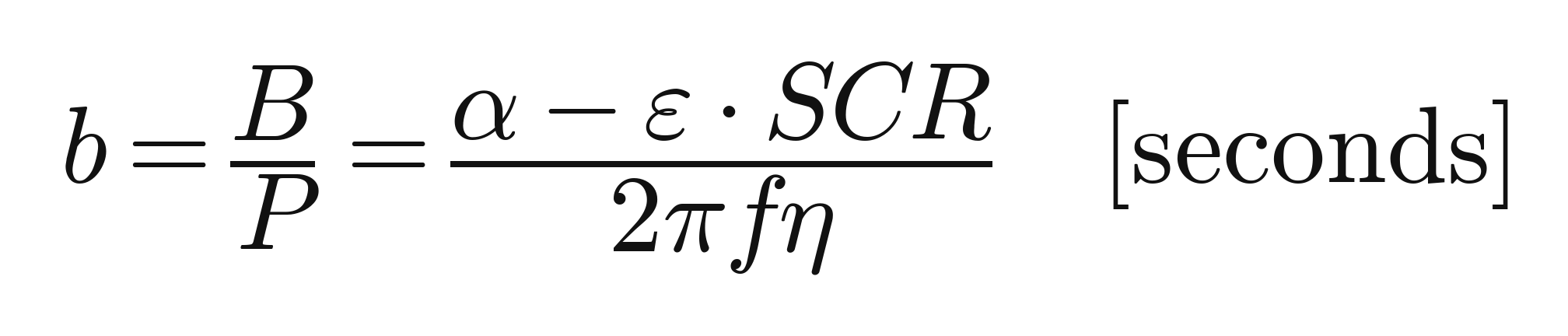
The buffering requirement per MW of training load has units of seconds – the good thing about that, is that it makes it directly comparable to the ride-through figure every UPS in a data centre building is already specified against. So that means it’s a number that a facilities engineer, an electrical engineer and a utility repr4esentative can all argue about in the same room.
If we go back to our example, and run our 100MW hall through it:
Swing depth α = 0.30 (NVIDIA’s own smoothing work quotes a 30% reduction in peak grid demand, so that’s a fair centre of the range).
Connection at short-circuit ratio 8, a realistic weak-ish 132kV position. ε = 1.5%.
Frequency 1Hz, the middle of the published band.
Round-trip efficiency 0.9.

Plugging in some more numbers revealed something I didn’t expect to work: NVIDIA’s GB300 NVL72 power shelves carry 65 joules of electrolytic capacitance per GPU, 72 GPUs to a rack, in a rack drawing about 132kW. That’s 35kJ per MW. My steel-derived rule says 32.
I’ll caveat about how much weight that figure should carry in my argument. I took f from the middle of a published band and α from NVIDIA’s own headline figure, so the check isn’t independent, and the sensitivity is quite brutal: at the 0.2Hz end the requirement is five times larger, at 3Hz it’s a third. A capacitor bank sized like NVIDIA’s is right for the fast end of the spectrum and short for the slow end.
Note also what the ε·SCR term does. Take the same example hall to a connection with a short-circuit ratio of 20 and the allowance swallows the entire swing; the storage requirement goes to zero. Grid stiffness and stored energy are substitutes.
So in simpler terms: you can buy your buffer in copper, or you can buy it in joules.
Ramp and circumstance
The capacitors solve the ripple. But they do nothing whatsoever about the other problem, which is what happens when something starts, stops, checkpoints or loses a node, and 100MW appears or vanishes as a step.
Usually, most utilities companies don’t regulate that with a spectrum. They regulate it with a ramp rate, in MW per minute, written into the connection agreement. If your load steps by ΔP and the network will only follow you at R, the deficit decays linearly and the energy you have to cover is:
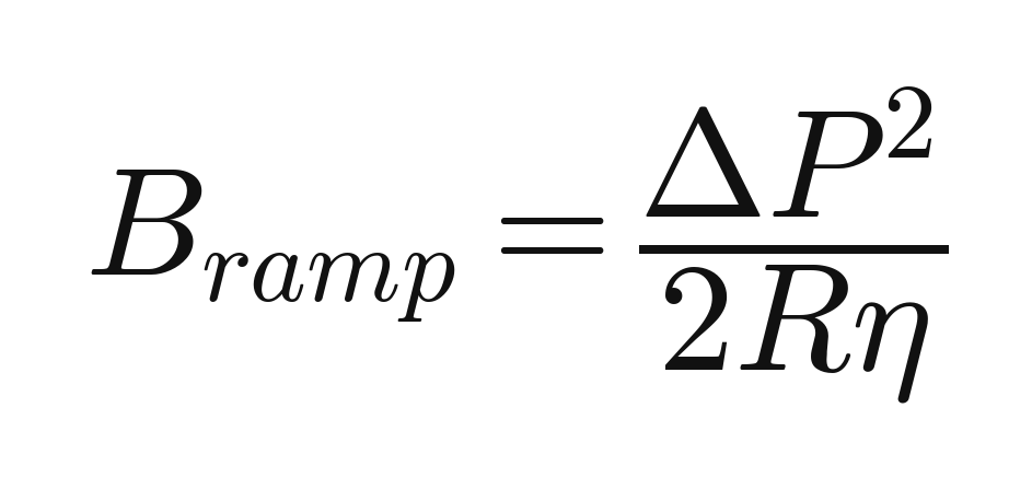
At a permitted 10MW/min, a 100MW step needs 9.3MWh. That’s 93kWh per MW, against 32 kilojoules per MW for the ripple. Ten thousand times.
Both numbers seem a bit intimidating, but are still completely buildable. 9.3MWh is a handful of Megapacks and an unremarkable line in a £500m large compute or hyperscale project.
But they are different machines, on different balance sheets, with different failure modes, and treating them as one procurement is how you end up with the situation Bloomberg reported earlier this month: batteries installed for stabilisation duty being replaced within weeks because they’re being cycled at a rate nothing in their warranty anticipated. A battery asked to chase a 1Hz ripple will destroy itself. But a capacitor asked to cover a two-minute ramp is9n’t even in the right order of magnitude.
What the steel industry actually knew, and what it can teach us
The transferable insight isn’t the implementation of the STATCOM, but probably more about the paperwork and the discussions about what it’ll actually do under load (before it’s built).
When a furnace applies to connect, it declares its Kst, its rating and the short-circuit power at its proposed connection point, and the network operator checks the arithmetic against a published planning level and says yes or no. The applicant pays for its own compensation. Everyone knows the number before tany capital is committed.
A data centre connection application often only declares megawatts, and that’s the whole disclosure. Given that the load in question can move a third of that figure in under a second, in a frequency band that talks directly to turbine shafts, this initially suggests to be an odd place to have stopped asking questions.
If I were redesigning the application form I’d want two more fields on it: swing depth as a fraction of contracted load, and the frequency band that swing occupies. Everything above falls out of those two, and neither is hard to measure; the operators already hold the telemetry, which is how the NVIDIA and Microsoft paper got written in the first place.
I’ll accept the limits of all this, as I’m sure I[‘ve butchered the theory with a lot of oversimplification. My ε transposition wants testing against real emission data before anyone puts it in a contract or quotes it verbatim. Swing depth and frequency vary enormously with model architecture, parallelism strategy and cluster size, and they’ll keep moving as training methods change; inference behaves nothing like this. A formula that assumes a clean sinusoid is also being very generous about a signal that is, in practice, a mess.
Behind the theory is a more stark reality, and one which may need to be thought about more if the country decides to re-industrialise. If we take Port Talbot’s furnace and our hypothetical AI training hall down the road - they’ll eventually approach the utility operator asking ffor the same favour. One of them will arrive with its homework done, its compensation costed and a hundred years of standards behind the number. The other will arrive with a megawatt figure and a smile.
And in that situation, I know which one I’d connect first.
TH